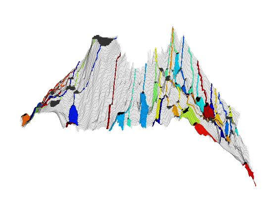
The purpose of the example is to demonstrate some of the functionality we have available for studying migration patterns and finding structural trapping. As an example, we consider the Utsira formation for which we will trace gravity lines, identify structural traps, and investigate how they are connected.

Contents

Load data

Make top-surface grid from a coarsened version of the Utsira formation

[grdecl,m] = getAtlasGrid('Utsirafm','coarsening',3);
G    = processGRDECL(grdecl{1});
Gt   = topSurfaceGrid(G(1));
meta = m{2}.meta;
data = abs(m{2}.data)';
data(data==0) = NaN;

Trace gravity lines on the top surface

To show the potential migration paths, we trace 'gravity' lines in the upward direction using a flux defined on a standard TPFA type connection

% Define flux
internal = all(Gt.faces.neighbors>0,2);
n1   = Gt.faces.neighbors(internal,1);
n2   = Gt.faces.neighbors(internal,2);
flux = zeros(Gt.faces.num,1);
flux(internal)= Gt.cells.z(n2) - Gt.cells.z(n1);
state = struct('flux',flux);
clear internal n1 n2 flux;

% Pick approximately five hundred cells and trace streamlines backward
% using the Pollock routine from MRST's streamlines module
mrstModule add streamlines
seeds = (1:ceil(Gt.cells.num/500):Gt.cells.num)';
S = pollock(Gt, state, [seeds, repmat([.5,.5],numel(seeds),1)], 'reverse', true);

% Make Cartesian grid for fast interpolation to surface
y = linspace(0,meta.cellsize*(meta.ncols-1),meta.ncols) + meta.yllcorner;
x = linspace(0,meta.cellsize*(meta.nrows-1),meta.nrows) + meta.xllcorner;
[X,Y] = meshgrid(x,y); clear x y;

% Collect streamlines in a long array separated by zeros and calculate the
% corresponding z-value by interpolating in the original meta data set.
% Afterwards, replace zeros by NaN's for use in plotting.
c = zeros(sum([cellfun(@length,S); numel(S)]),3);
i = 1;
for k=1:numel(S)
   nsl = length(S{k});
   c(i:i+nsl-1,1:2) = S{k};
   i = i+nsl+1;
end
c(:,3) = interp2(X,Y,data, c(:,1), c(:,2));
c(c==0)=NaN;

% Use the original meta data to surf make the surface, but offset the plots
% slightly to distinguish the surface and the gravity lines
figure(1),clf
surf(X,Y,data+1),shading interp
hold on
plot3(c(:,1),c(:,2),c(:,3)-1, 'k-', 'LineWidth', 1);
hold off
view(70,50), axis tight, set(gca,'ZDir','reverse');

Find trapping structure

We find all traps corresponding to local maxima on the top surface. The traps are categorized as different levels. A level-1 trap contains one local maximum point; a level-2 trap contains at least two level-1 traps and hence at least one spill point; a level-3 trap contains at least two level-2 traps; and so on. As part of finding the trapping structure, we construct a new top-surface grid for which the topography inside the level-1 traps have been replaced by a flat surface at the depth of the corresponding spill point.

% Check for existence of the MATLAB graph library
checkBGL();

ts=findTrappingStructure(Gt);

% Plot the new top-surface grid on top of the old one to show the location
% of traps
clf, subplot('position',[.025 .025 .95 .95]);
plotGrid(Gt,      'FaceColor','r','EdgeAlpha',.1)
plotGrid(ts.Gtop, 'FaceColor','y','EdgeColor','none');
view(92,40), axis tight off, set(gca,'ZDir','reverse');

Trap level 1: 102 traps identified
Trap level 2: 13 traps identified
Trap level 3: 1 traps identified

Show the flat parts of the grid

cla
plotGrid(ts.Gtop,'FaceColor','none','EdgeAlpha',.1)
plotGrid(ts.Gtop, ts.z_spill_loc>0, 'EdgeAlpha', .1)

Show the traps on different levels in different colors

cla
plotGrid(ts.Gtop,'FaceColor','none','edgeAlpha',0.1)
nt  = numel(ts.trap_level);
col = hsv(nt);
for k=nt:-1:1
   cell_list = [];
   for i=1:size(ts.trap_level{k},2)
      cell_list = [cell_list; find(ts.trap_level{k}(:,i)>0)]; %#ok
   end
   plotGrid(Gt, cell_list, 'FaceColor', col(k,:),  'EdgeAlpha',.1);
end
colormap(col); cbh=colorbar('horiz'); caxis([0 nt]+.5);set(cbh,'XTick',1:nt);
view(100,70)

All the CO₂ that accumulates in a trap must come from the trap's drainage area that consists of all cells that have an updip connection to the trap. We show the drainage/accumlation area of the different traps defined as the cells whose spill paths lead into the corresponding local top point. A spill path is the path that the CO₂ will follow in its upward migration when injected infinitesimally slow from a given point

clf, subplot('position',[.025 .025 .95 .95]);

% To find the drainage area, we construct a directed graph from the gravity
% flux, make this graph bi-directional along each edge, and then compute
% the connected components.
C       = maxTPFAGravityMatrix(Gt);
[ci,ss] = components(C+C');  assert(max(ci)==numel(ts.top))

% Set a unique random color for each trap
p  = zeros(length(ts.top),1);
nt =  sum(ts.istrap);
p(ci(ts.top(ts.istrap))) = randperm(nt)';

% Plot grid, drainage areas for traps, and the local top points
plotGrid(Gt, 'FaceColor','none', 'EdgeAlpha', .05)
plotCellData(Gt,p(ci), p(ci)>0, 'EdgeColor', 'none');
plotGrid(Gt,ts.top(ts.istrap), 'FaceColor',[.45 .45 .45],'EdgeAlpha',.1);
axis tight off, view(85,50), colormap(jet(nt));

Find trap connections (river system)

The CO₂ is typically injected low in the formation and if we disregard all other trapping mechanisms, the CO₂ will migrate upward until it encounters a structural trap. Once a trap is filled, the CO₂ will spill over and start to migrate upward along a spill path and either reach the top of the formation or start to accumulate in a more shallow trap until this trap spills over, and so on. We start by computing the connections between the traps.

mrstModule add coarsegrid

trap_con    = findTrapConnections(Gt, ts.z_spill_loc);
cell_lines  = trap_con.cell_lines;
traps       = trap_con.traps;
leaf_lines  = trap_con.leaf_lines;
leaf_traps  = trap_con.leaf_traps;
trap_matrix = trap_con.trap_matrix;

Start find rivers

If we invert the axis, the structural trapping may be thought of as water flowing down in a terrain consisting of impermeable soil. The water will collect in ponds and small lakes that are possibly connected by natural watercourses (rivers).

% Find connection stucture of the river network
comp = components(trap_matrix+trap_matrix');
trap_comp=nan(size(traps));

% Make vectors representing each independent waterway
p = randperm(max(comp));  % to avoid the proximity of similar colors
for i=1:numel(comp)
    trap_comp(i==traps)=p(comp(i));
end
cc=[ts.Gtop.cells.centroids,ts.Gtop.cells.z];
[x,y,z] = deal([]);
for i=1:numel(cell_lines);
   x = [x; cc(double(cell_lines{i}),1); NaN]; %#ok
   y = [y; cc(double(cell_lines{i}),2); NaN]; %#ok
   z = [z; cc(double(cell_lines{i}),3); NaN]; %#ok
end

% Plot the 'lakes' and the watercourses
clf, subplot('position', [.025 .025 .95 .95]);
plotCellData(ts.Gtop,trap_comp)
plotGrid(ts.Gtop,'FaceColor','none','edgeAlpha',0.1)
hold on
plot3(x,y,z, 'k', 'LineWidth', 2)
hold off
view(280,40), axis tight off; set(gca,'ZDir', 'normal');

As our last example, we will look at leaf nodes in our trapping system, i.e., traps that only have outgoing 'rivers'. The leaf traps are shown in white color. The drainage areas and the resulting migration path are given a unique color so that one can trace the migration of CO₂ upward until it either leaves the formation or reaches a higher trap that accumulates CO₂ from multiple leaf traps. All traps that are not leaf traps are shown in dark gray.

% Plot traps and grid
cla
plotGrid(ts.Gtop, ts.z_spill_loc>0, 'EdgeColor', 'none', 'FaceColor',[.25 .25 .25])
plotGrid(ts.Gtop, 'FaceColor', 'none', 'EdgeAlpha', .1)

% Find leaves and the corresponding traps
[ll, tc, dc] = deal([]);
C    = maxTPFAGravityMatrix(ts.Gtop);
nll  = numel(leaf_lines);
p    = randperm(nll);
lvol = zeros(nll,1);
tic
for k=nll:-1:1
   % extract the leaf line out of the trap
   ll  = [ll; leaf_lines{k}', p(k)*ones(length(leaf_lines{k}),1)]; %#ok

   % find all cells in the given trap
   t_cells = find(traps ==leaf_traps{k});
   tc = [tc; t_cells]; %#ok

   % find all cells in the drainage region of the leaf
   cc = find( dfs(C', double(t_cells(1))) >0);
   dc  = [dc; cc, p(k)*ones(length(cc),1)]; %#ok

   % calculate the leaf volume
   cc = find( dfs(C, double(t_cells(1)))>0 );
   lvol(k) = sum((ts.Gtop.cells.z(cc) - Gt.cells.z(cc)).*Gt.cells.volumes(cc));
   disp(['Leaf volume : ', num2str(lvol(k))]);
end

% Plot leaves and the deepest traps
plotCellData(ts.Gtop, [ll(:,2); dc(:,2)], [ll(:,1); dc(:,1)], 'EdgeColor', 'none');
plotGrid(ts.Gtop, tc, 'EdgeColor', 'none', 'FaceColor', 'w');
view(95,20), axis tight off; set(gca,'ZDir', 'reverse');

Leaf volume : 618782.3458
Leaf volume : 1920205.7847
Leaf volume : 0
Leaf volume : 33295634.1306
Leaf volume : 34577258.0053
Leaf volume : 28458992.5049
Leaf volume : 136488585.5204
Leaf volume : 820247394.6633
Leaf volume : 381407666.5635
Leaf volume : 975677262.5204
Leaf volume : 812477042.3271
Leaf volume : 13273947.4493
Leaf volume : 812032999.8997
Leaf volume : 921435649.9908
Leaf volume : 849094847.046
Leaf volume : 361006825.2235
Leaf volume : 9101232.1556
Leaf volume : 509961.9253
Leaf volume : 36649535.63
Leaf volume : 15594.5838
Leaf volume : 496026164.2495
Leaf volume : 7022319093.149
Leaf volume : 1468444523.9203
Leaf volume : 99286419.5772
Leaf volume : 1469819977.0619
Leaf volume : 2572532.6835
Leaf volume : 228483848.0456
Leaf volume : 1469819977.0619
Leaf volume : 7519927861.7073
Leaf volume : 1009105.2054
Leaf volume : 18805622.7009
Leaf volume : 2621476253.2478
Leaf volume : 1686896.3595
Leaf volume : 1207744737.7059
Leaf volume : 3862613.6834
Leaf volume : 270895768.0561
Leaf volume : 1505263255.3188
Leaf volume : 1505263255.3188
Leaf volume : 582974.0581
Leaf volume : 581524995.8565
Leaf volume : 1218254059.2199
Leaf volume : 34567037.3357
Leaf volume : 1220898307.2355
Leaf volume : 581336917.8887
Leaf volume : 745338740.1382
Leaf volume : 40227970.7599